Map Matching Part 1 - GPS, Maps and Graphs

This series of articles will look into the subject of map matching, providing foundational knowledge. It examines the core concepts and inherent challenges within this domain, and details a comprehensive process for generating a synthetic dataset. I’ll then extends to exploring various map matching algorithms and a comparative evaluation of their performance, utilizing the dataset constructed.

GPS Data

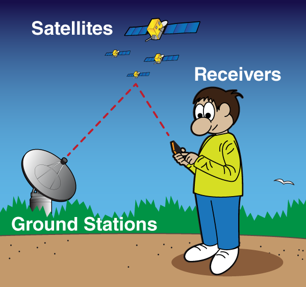
While we often take for granted the availability of GPS on most of our mobile devices, in the background, this is actually quite a complex feat that is somehow available to us, essentially for free. Originating from U.S. military research in 1973 and made open to civilians in 1980 [1], GPS, short for Global Positioning System, accurately describes itself: “Global” means it’s available worldwide, “Positioning” means it’s designed to determine locations, and “System” signifies that it requires multiple components. Let’s explain it in a hand-wavy way: there are satellites in space whose locations are known, and some ground stations on Earth whose positions are also known. These two communicate to ensure both satellites and ground stations are precisely where we expect them to be. Now for the last part: the users’ devices, which contain a GPS receiver chip. This receiver is able to obtain signals from the satellites and triangulate its location based on multiple parameters received from them.

https://spaceplace.nasa.gov/gps/en/ [2]

GPS receivers can provide all kinds of useful information, but for our discussion, only five matter: longitude, latitude, bearing (or heading), accuracy, and timestamp. Longitude, latitude, and timestamp are pretty self-explanatory. Bearing, or heading, is the angle measured in degrees in a clockwise direction from true north [3]. Usually, bearing indicates an angle to a specific place, while heading is the angle of the device itself. Accuracy is more of a probability field - it’s the radius (in meters) within which there is a 68% chance that the actual signal is located [4]. This means if we receive an accuracy value of 3 meters alongside latitude and longitude, there is a 68% chance that the actual location is within 3 meters of the received coordinates.

Noisy Measurements

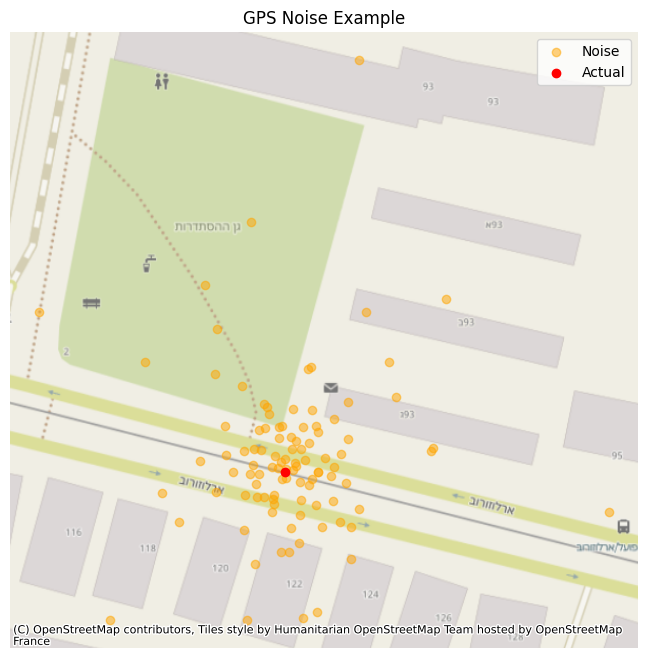
GPS measurements contain noise due to multiple factors. Atmospheric interference, signals that can bounce off objects, geometric arrangement of visible satellites, satellite clock inaccuracies and minor errors in orbital data also contribute to measurement noise. Receiver quality and internal processing algorithms further influence the level of noise in the final output. Meaning, even if we stand still, our GPS measurement may think we continue moving all the time. Latitude and longitude typically have errors in the range of 5–10 meters for standard receivers under open sky conditions; high-accuracy receivers can achieve around 1 meter. Altitude measurements are generally less precise, with errors potentially reaching 10–20 meters or more. Heading accuracy can vary significantly, ranging from a few degrees to tens of degrees, especially at low speeds. Bearing accuracy depends on the accuracy of the start and end points and the distance between them. Speed accuracy is generally better than positional accuracy, potentially within a few tenths of a meter per second. [3]

Maps and Graphs

Geographic maps visually represent spatial data, displaying features like points, lines, and polygons with associated coordinates and attributes. Think of a map showing buildings (polygons), rivers (lines), and landmarks (points). Graphs, however, model the relationships between these geographic entities. In a graph, nodes represent discrete locations or points of interest, while edges represent the connections or relationships between them. For instance, a road network is perfectly suited for graph representation: intersections become nodes, and the roads connecting them become edges. This graph structure is then overlaid on a geographic map. This powerful combination allows us to apply advanced graph algorithms to solve spatial problems directly on geographic data, enabling applications like efficient routing or complex network analysis. Now, while maps provide the visual context and graphs offer the relational structure, there’s a crucial step to bridge the gap between noisy, real-world GPS measurements and the clean, structured digital road network. This is where map matching becomes handy.

What is Map Matching

Map matching is a crucial process in location-based services, addressing the inherent inaccuracies present in raw GPS data by aligning recorded coordinates with a road network. At its core lies the concept of “snapping,” where individual GPS points are associated with the most probable road segment. This association is not solely based on proximity, different algorithms consider a multitude of factors, including the spatial closeness of the point to potential road segments, the direction and speed of travel inferred from the sequence of points, and the topological connectivity of the road network. By intelligently “snapping” these noisy measurements to the underlying infrastructure, map matching algorithms generate a more accurate and coherent representation of the traveled path, enabling reliable navigation, traffic analysis, and various other applications. A simple example of the importance of such a thing is your everyday scenario - you’re driving and your navigation app loses GPS signal in a short tunnel. Without map matching, the software would struggle, likely misplacing your vehicle by hundreds of meters. However, map matching would have already aligned your position to a specific road. Assuming the tunnel has no intersections, the system predicts your continued movement along that same road, using your car’s speed and calculations (like linear algebra) to maintain an accurate location estimate.

Implementation First Step - Map to Graph

In order to properly implement and learn map matching algorithms, we first need to have a map and a matching graph. Lets have a quick look on how we can accomplish that. We kick things off using the pyrosm library, which is handy for working with OpenStreetMap (OSM) data (basically a massive, free map of the world).

Here’s how we pull out the raw network parts:

import os
from pyrosm import OSM
import igraph as ig
import numpy as np

# Assuming map_path and crop_bounding_box are set up earlier
# map_path points to our downloaded OSM file
# crop_bounding_box lets us focus on a specific area if needed

osm = OSM(map_path, bounding_box=Config.crop_bounding_box)
# Get all the road segments and their intersections
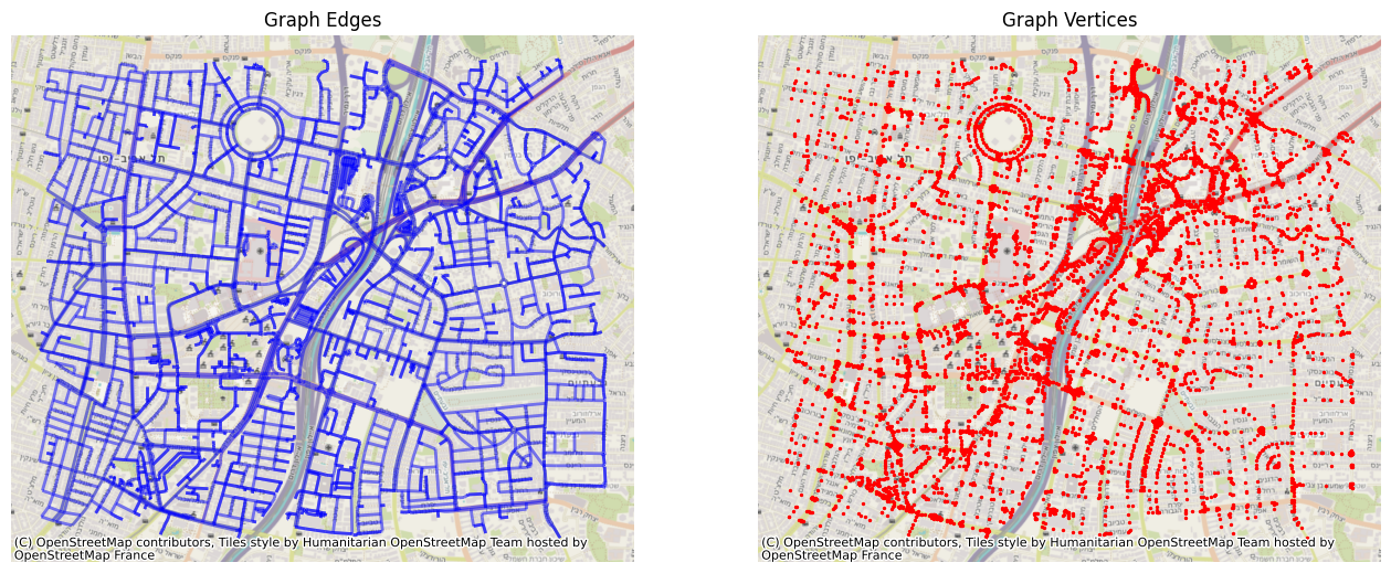
nodes, edges = osm.get_network(nodes=True, network_type='driving')

What’s happening above is OSM loads our map file, and then get_network sifts through it to find all the bits that make up the “driving” network - that’s our roads and where they meet. The nodes are essentially the intersections or endpoints, and edges are the actual road segments connecting them. (Also, don’t worry, the code in the repo also includes downloading the map and setting the configuration value for the bounding box. Just a bit boring to add that in here as well).

Once we have these nodes and edges from the raw map data, we hand them over to igraph chosen mostly because of performance. This step builds the actual graph structure we need:

# Convert the extracted nodes and edges into an igraph object
graph = osm.to_graph(nodes, edges, graph_type='igraph')

This line is the core of the transformation. It takes those raw map elements and creates a proper graph where our intersections are vertices and the road segments are edges. The cool part is that pyrosm automatically carries over useful information from the OSM data, like the road’s name or its geometry (the actual shape of the road segment). We then take that geometry and use it to calculate things like the road’s bearing, and we also clean up other attributes like maxspeed, ensuring every edge has the data we need for later calculations.

# Loop through every edge (road segment) in our new graph
for edge in graph.es:
# Calculate the bearing (direction) of the road segment
edge['bearing'] = self.calculate_bearing(edge)
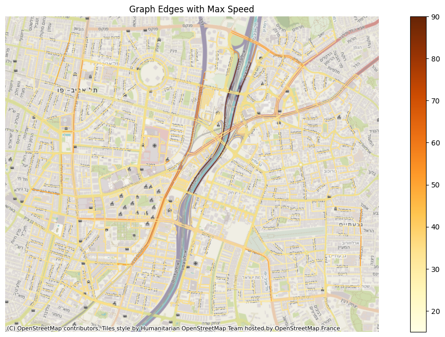
# Set a default maxspeed if it's missing, otherwise convert to float
if edge['maxspeed'] is None:
edge['maxspeed'] = 35.
else:
edge['maxspeed'] = float(edge['maxspeed'])

By adding bearing and cleaning up maxspeed, we’re essentially enriching our graph. It’s not just a bunch of connected lines anymore; it’s a smart representation of the road network that understands directionality and speed limits. This robust graph is then ready for all sorts of advanced uses, especially when we get to the tricky business of map matching.

Resources

Code

https://github.com/ornachmias/map_matching

References

[1] https://en.wikipedia.org/wiki/Global_Positioning_System

[2] https://spaceplace.nasa.gov/gps/en/

[3] https://www.lifewire.com/what-is-bearing-in-gps-1683320

[4] https://developer.android.com/reference/android/location/Location#getAccuracy()