This series of articles will look into the subject of map matching, providing foundational knowledge. It examines the core concepts and inherent challenges within this domain, and details a comprehensive process for generating a synthetic dataset. The discussion then extends to exploring various map matching algorithms and a comparative evaluation of their performance, utilizing the dataset constructed.

Part 1

Generating a Dataset

Having established what map matching is and why it’s necessary, our next step is to explore the algorithms that perform this task. However, before evaluating these algorithms, we first require a suitable dataset. The following section details the code used to generate both augmented noisy GPS data and its corresponding ‘actual’ non-noisy counterpart.

Synthetic Data

Following the initial graph construction, the next phase focuses on generating augmented data based on this graph. The dataset file encapsulates all logic for this data generation process. While it might be more efficient to work in a vectorized form on the data, I’ve decided to work iteratively for numerous reasons: The code is more readable, which is important since I assume no previous knowledge is needed to read this article.

Intuitively, it simulates the way we expect the GPS to work.
Performance is not much of a concern at this point.
If you decide to take it to production and generate points over an entire country, I recommend that you take the time to re-write it in vectorized form to improve performance.

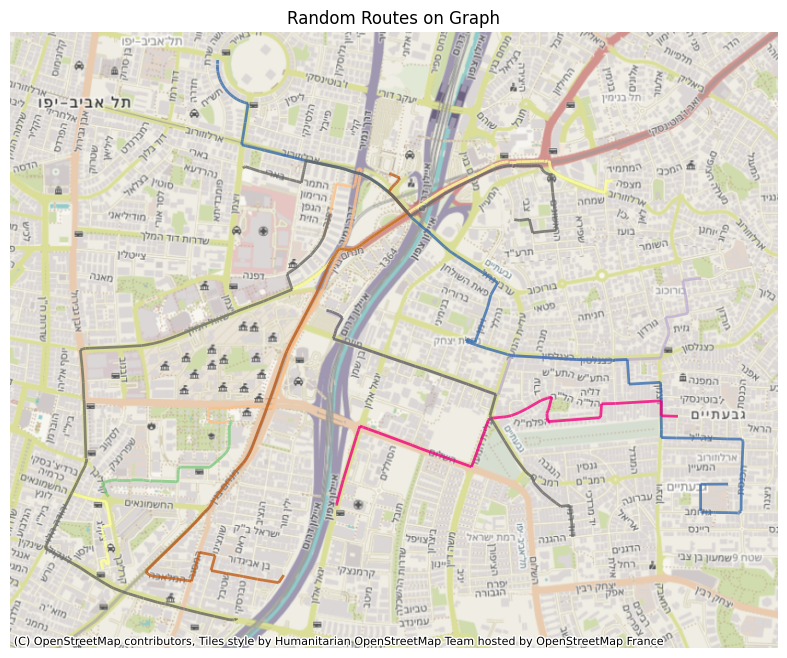
Select a Route

The first step is to generate a realistic route from the graph. This route serves as the ground truth that our algorithms will try to reconstruct. The process begins with the selection of source and target vertices. These are chosen randomly from the graph, with the limitation that they should be separated by a minimum distance of 100 meters. This constraint is implemented to prevent trivial routes, such as those where the origin and destination are on the same edge. For this distance calculation here and in the next steps, the coordinates are projected to an appropriate local CRS to ensure geographic accuracy, a methodology detailed in my previous post. Once suitable source and target vertices are identified, the get_shortest_path method, provided by the igraph package, is employed to determine the sequence of edges forming the optimal path between them. Some of you might notice a problem with those sources and targets - they will never be at the middle point of an edge. While data points for data generation are generated across all of the route’s edges, this characteristic of start and end points being on nodes is considered acceptable for our purposes. The rationale is that the point-matching process applies to all generated data points along the route, and the specific location of the route’s two endpoints has a limited impact on the overall augmented dataset.

Points’ Timestamps

With the route itself established, the arguably more tricky task is to determine the timestamps for our simulated GPS sampling points along this path. While many applications are configured to send location data at fixed intervals (say, every X seconds), the reality of server-side data is often less predictable. To create a dataset that reflects it, we need to simulate how far a user would travel in variable time-frames, rather than strictly uniform ones. The challenge is that real-world data isn’t always clockwork. An app might be set to send GPS updates every few seconds, but several factors can lead to data being missing, delayed, or ill-synchronized. For example, driving through an area with no cellular reception, like a tunnel, can interrupt transmission. In other instances, a user might switch to another app (hopefully Spotify and not iMessages) and when background data collection isn’t permitted, it’ll temporarily halt updates. On a more technical note, slight drifts between satellite and receiver clocks can also cause minor deviations in the actual sampling intervals [1]. Our dataset needs to reflect these common scenarios. To model these variations, I’ve chosen to generate the time intervals between samples using a randomized approach based on a normal distribution. We’re using a mean interval of 4 seconds with a standard deviation (sigma) of 3 seconds. This setup means most time gaps between samples will naturally fall between 1 and 7 seconds. I’ve also implemented a minimum interval of 1 second to prevent multiple samples from effectively occurring at the same instant.

Driving Speed

Beyond just the route, another key variable influencing both a driver’s location over time and the perceived accuracy of GPS bearing measurements is the driving speed. Since we’re not working with live measurements, we need to simulate these speeds. The most sensible starting point for this is the posted speed limit for each road segment. We take this information from OpenStreetMap’s maxspeed attribute. (For segments where this data is missing, we already had a fallback strategy discussed in previous post). This maxspeed then becomes our base for our speed simulation. For each edge in our graph, we model the driving speed by drawing a random value from a normal distribution. The mean of this distribution is set to the edge’s maxspeed value, and I’ve chosen a standard deviation equal to half of that mean. This touch of randomization is our way of mimicking real-world driving: the flow of traffic, individual driving styles, and other on-the-road variables. As an example, consider a road segment with a maxspeed of 90 km/h. Our model uses a mean of 90 km/h and sigma of 45 km/h, which can generate realistic speeds. This includes everything from very slow travel (e.g. traffic jam) up to speeds around the 90 km/h limit. It also allows for drivers reasonably exceeding this limit - for instance, speeds up to around 135 km/h are within one standard deviation. While the model will mostly generate speeds closer to the mean, it doesn’t entirely rule out those more… enthusiastic drivers (like the 232 km/h scenarios that occasionally make headlines [2]), as these would represent rarer values further out in the distribution’s tail.

Coordinates

Alright, with our route charted and speeds for each segment determined, we’re ready to generate the actual sequence of GPS points along this path. We begin our journey with a relative timestamp of zero. This means we’re not tied to a specific real-world start time, instead, the absolute “when” of the route can be decided by whatever application eventually uses this data. It keeps things nice and flexible. To place each data point, we effectively “drive” along our route, edge by edge. For each segment, we interpolate points based on two main ingredients: the simulated speed for that particular edge and our series of (deliberately varied) sampling timestamps. The geometric magic for this is handled by the line_interpolate_point function from the shapely package. Essentially, you provide this function with the start and end coordinates of an edge, the speed assigned to it, and a specific time offset (from our sampling timestamps, representing time elapsed along that edge), and it calculates the precise coordinates where that sample point would fall.

Accuracy

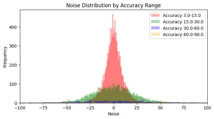
Now, let’s talk about GPS accuracy. For each simulated location point, I also need an associated accuracy value. This figure usually indicates a radius in meters around the reported coordinates, representing a 68th percentile confidence level [3]. Essentially, how much wiggle room there is in that fix. As you might guess, a whole host of factors play into how good (or bad) this accuracy figure can be. We’re talking satellite positions, how tall the buildings are around the device, signal strength, atmospheric conditions, and more [4]. While diving deep into all those variables is a fascinating journey (though perhaps a longer one than you’d initially sign up for), our aim here is to generate values that feel realistic for our dataset. To achieve this, I’ve set up a system based on four predefined accuracy ranges, reflecting different real-world conditions:

3–15 meters: Pretty good signal, representing optimal or near-optimal conditions.
15–30 meters: Decent, but perhaps some minor interference - let’s call these sub-optimal conditions.
30–60 meters: Now we’re getting into noticeably noisy values.
60–90 meters: This represents more significant signal degradation, the kind of interference I’ve occasionally spotted in production databases.

To decide which of these ranges a particular sample’s accuracy will come from, I use a weighted selection approach with the following probabilities: [0.7, 0.25, 0.04, 0.01]. So, most of the time (70%) we’ll be in optimal conditions, but we’ll still get a sprinkle of the less ideal scenarios. Once a range is selected based on these weights, an actual accuracy value is then picked uniformly at random from within that specific range.

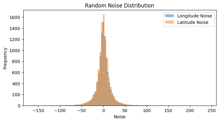
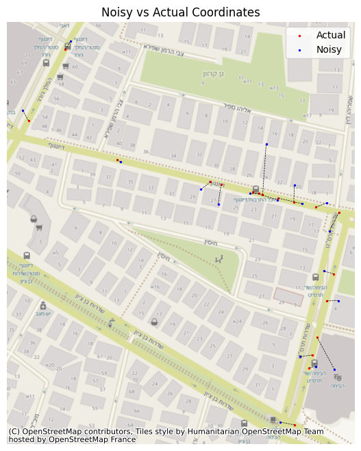
Coordinates Noise

So now that we’ve got the samples and an accuracy for each one, we can start introducing noise to each set of coordinates. This noise depends upon the accuracy we’ve set to the point, since the samples can be in any place inside this horizontal measurement, based on normal distribution. So we set our noise with mean 0 and std of the accuracy, and we generate the noise. The overall distribution of noise will seem like one single normal distribution, but when we separate it by the accuracy, we’ll see its multiple normal distributions behaving differently from one another, due to our parameters and number of samples in each group. With our sample points and their GPS accuracy established, it’s time to introduce some realistic positional noise. The amount of noise added to each coordinate is directly tied to its pre-assigned accuracy value. We model this uncertainty by assuming the error around the initially calculated location follows a normal distribution. Specifically, for each coordinate, we generate noise from a normal distribution with a mean of zero and a standard deviation that matches the point’s specific accuracy value (in meters). Interestingly, if you looked at all the applied noise collectively, it might resemble a single normal distribution. However, it’s more nuanced than that. When you consider the noise based on our defined accuracy tiers (optimal, sub-optimal, etc.), it becomes clear that the overall effect is a composite of multiple distinct normal distributions. Each tier contributes a distribution with a different spread (its standard deviation), shaping a more varied and ultimately more realistic scatter of GPS points.

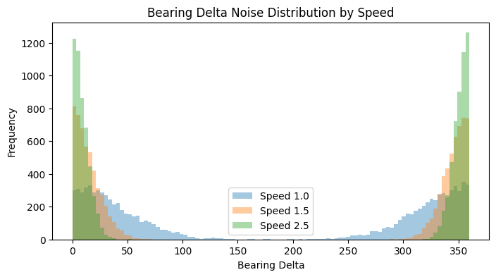
Bearing Noise

Now for the final step - the bearing. The bearing is calculated from successive position fixes, so if the device is moving slowly, the distance between these fixes is tiny, making the direction calculation quite sensitive to small GPS position errors [5]. Reflecting this, our model applies a more substantial random noise when the simulated speed drops below 1.5 m/s, drawing from a normal distribution with a mean of 0 and a hefty standard deviation of 45 degrees. Once the speed picks up beyond that 1.5 m/s threshold, GPS bearing typically becomes more stable. The accuracy generally improves as the vehicle moves faster because the distance between position fixes increases, making the direction calculation less susceptible to minor positional noise [6]. Our simulation mirrors this by calculating the noise’s standard deviation as inversely proportional to the speed (using a scaling factor of 30.0 degrees*m/s). However, since no GPS is perfect, even at higher speeds, we ensure there’s always a touch of uncertainty by setting a minimum noise standard deviation of 2.0 degrees. This generated noise is then added to the true bearing, and the result is neatly wrapped to stay within the 0–360 degree range, giving us our final, realistically noisy, bearing.

Summary

In this initial part of our series on map matching, we’ve focused on discussing the essential concepts. This foundational understanding, coupled with the carefully prepared dataset, paves the way for the second part of our series, where we will delve into various map matching algorithms and assess their performance.

Resources

Code

https://github.com/ornachmias/map_matching

References

[1] https://www.researchgate.net/post/GPS_data_recording_at_equal_time_intervals_impossible

[2] https://www.ynet.co.il/news/article/SkJ4tTdaw

[3] https://developer.android.com/reference/android/location/Location#getAccuracy()

[4] https://web.stanford.edu/group/scpnt/pnt/PNT15/2015_Presentation_Files/I15-vanDiggelen-GPS_MOOC-Smartphones.pdf

[5] https://www.ardusimple.com/how-gps-can-help-you-measure-the-real-heading-of-your-vehicle/

[6] https://medium.com/anello-photonics/mastering-true-north-5-ways-to-determine-your-absolute-heading-d63fc3543c0