Map Matching - The Viterbi Snapper

In the map matching series, we built our way from a naive nearest-edge baseline up through weighted scoring and topological bias, ending with a hybrid algorithm that blends both approaches depending on GPS accuracy. At the end of Part 3, I mentioned Hidden Markov Models as a direction worth exploring. Well, here it is - covering what map matching with Viterbi is, the theory behind it, and a step-by-step implementation.

What is Map Matching with Viterbi?

Every algorithm from the previous series shared the same fundamental assumption: each GPS point is matched independently. You look at the GPS location, find nearby edges, pick the best one, and move on. This is fast and intuitive, but it has a structural flaw - once you commit to the wrong edge, there’s no mechanism to go back.

Consider a vehicle turning from a main road onto a small side street. The GPS point at the turn is noisy and lands geometrically closer to the main road. A greedy algorithm snaps it to the main road. The next few points are clearly on the side street, so they snap correctly, but the committed error lives forever in the output.

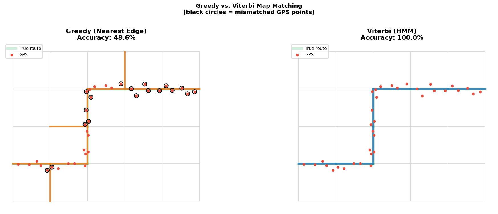
The Viterbi snapper takes a different stance. Instead of matching one point at a time, it finds the single most likely sequence of road edges that explains the entire GPS trace, jointly. The question changes from “what is the best edge for this point?” to “what is the best path through the road network that explains all these points together?”

This is the map matching problem reframed as a sequence decoding problem and solving it requires two things: a probabilistic model of how GPS observations relate to road edges, and an efficient algorithm to find the globally optimal sequence over that model.

Hidden Markov Models

A Hidden Markov Model (HMM) is a framework for reasoning about systems where we observe noisy outputs of a hidden, underlying state. The hidden state evolves over time according to fixed transition probabilities, and at each step we receive an observation whose probability depends only on the current hidden state.

Formally, an HMM consists of:

• A set of hidden states S = {s₁, s₂, …, sₙ}
• A set of observations O = {o₁, o₂, …, oₘ}
• An initial state distribution π, where π(i) = P(state at t=0 is sᵢ)
• A transition matrix A, where A[i][j] = P(state at t is sⱼ | state at t-1 is sᵢ)
• An emission function B, where B(i, oₜ) = P(observing oₜ | current state is sᵢ)

Given a sequence of observations, the central question is: what sequence of hidden states most likely produced them? The Viterbi algorithm answers this exactly.

Mapping the Problem

In the map matching context:

HMM concept	Map matching meaning
Hidden states	Road edges in the road network graph
Observations	GPS points (longitude, latitude, heading)
Emission probability	P(GPS point | vehicle is on this edge)
Transition probability	P(moving to edge B | currently on edge A)

Given a GPS trace of N points, we want to find the sequence of edges E₁, E₂, …, Eₙ that maximizes:

P(E₁, …, Eₙ | GPS₁, …, GPSₙ) ∝ P(GPS₁ | E₁) × ∏ P(GPSₜ | Eₜ) × P(Eₜ | Eₜ₋₁)

This joint probability is what the Viterbi algorithm maximizes efficiently using dynamic programming.

Emission Probability

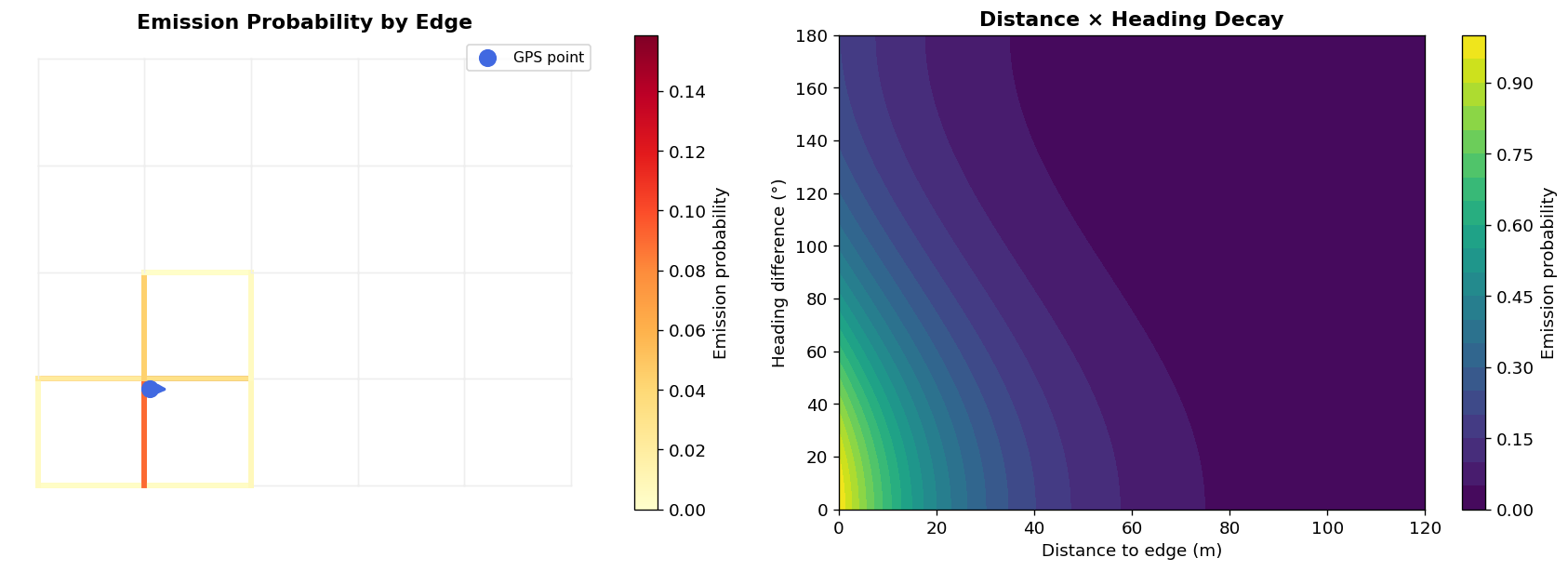
The emission probability answers: given that the vehicle is on this road edge, how likely is this GPS observation?

Two factors determine this:

Distance: How far is the GPS point from the candidate edge? A vehicle on that edge could plausibly produce a GPS reading a few meters away due to noise, but 200 meters away is much less likely.

Heading: Does the vehicle’s direction match the direction of the candidate edge? A GPS point 10 meters from an edge but aligned with its direction is far more convincing than one 5 meters away but pointing the wrong way.

These combine into a single exponential decay:

P(GPS | edge) = exp(-C_dist × distance - C_heading × heading_penalty)

Where the heading penalty is 1 - cos(angle_diff): zero when perfectly aligned, 2 when pointing exactly opposite. The cosine formulation is smooth and naturally handles the 0°/360° wraparound.

angle_diff_rad = np.radians(np.abs(segment_bearings - obs_heading))
heading_penalty = 1.0 - np.cos(angle_diff_rad)

probs = np.exp(
    -em_distance_factor * dists
    -em_heading_factor * heading_penalty
)

The two constants control the decay rate. A higher heading factor means the algorithm cares more about direction alignment, a higher distance factor makes it more sensitive to spatial proximity. In practice, setting the heading factor much higher than the distance factor encodes the intuition that being directionally wrong is a stronger signal of a mismatch than being a few meters off.

Only edges within a maximum distance threshold are evaluated as candidates. This is essential for performance, with tens of thousands of edges in a city graph, you can’t compute emission probabilities for all of them at every point.

Transition Probability

The transition probability answers: given the vehicle was on this edge, how likely is it to now be on that edge?

This is computed once, upfront, from the graph topology. For each edge, we examine its outgoing neighbors, the edges reachable by continuing to drive forward, and assign probabilities based on two factors:

Stay vs. move: If an edge is short, the vehicle probably crossed it between GPS samples, so move_probability is high. If an edge is long, the vehicle is likely still on it, so stay_probability is high. The vehicle either stays on the same edge (self-loop) or moves to a neighbor.

Turn angle preference: Not all neighbors are equally likely. A straight continuation gets higher probability than a sharp turn, and a U-turn gets nearly zero. This is encoded as exp(-angle_importance × |angle_diff|).

move_probability = min(avg_position_distance / edge_length, 0.5)

# Self-loop: staying on the same edge
transition[edge_idx][edge_idx] = 1.0 - move_probability

# Moving to neighbors, weighted by turn angle
angles = np.array([angle_diff for _, angle_diff in neighbors])
weights = np.exp(-angle_importance * np.abs(angles))
normalized_probs = (move_probability * weights) / weights.sum()

Lookahead: The transition matrix can be raised to a power before use, effectively compressing multi-hop paths into a single matrix. If GPS points are sparsely sampled, the vehicle may have crossed two edges between observations. Lookahead handles this without changing the Viterbi structure.

The result is stored as a sparse CSR matrix. The road network is highly sparse - each edge connects to only a small set of neighbors, so this representation is both memory-efficient and fast to traverse.

The Viterbi Algorithm

With emission and transition probabilities defined, the Viterbi algorithm solves the sequence decoding problem using dynamic programming.

Initialization

For the first GPS point, compute emission probabilities for all nearby edges. Let these form the initial state vector V₁:

V₁[e] = P(GPS₁ | edge e)   for all candidate edges e

Forward Pass

For each subsequent GPS point t, compute the best score for each candidate edge j:

V_t[j] = max_i( V_{t-1}[i] × T[i][j] ) × P(GPS_t | edge j)

In words: the probability of being on edge j at time t is the best combination of “probability of being on edge i at t-1” × “probability of transitioning from i to j” × “how well this GPS point fits edge j”. We record the predecessor i that achieved this maximum - this is the back-pointer.

for i, idx in enumerate(prev_active_states):
    val = prev_scores[i]
    neighbors = transition.indices[transition.indptr[idx]:transition.indptr[idx+1]]
    probs = transition.data[transition.indptr[idx]:transition.indptr[idx+1]]

    for k, neighbor in enumerate(neighbors):
        trans_score = val * probs[k]
        if trans_score > next_scores[neighbor]:
            next_scores[neighbor] = trans_score
            back_pointers[neighbor] = idx  # best predecessor

After processing all neighbors of all active states, multiply in the emission probabilities for the current GPS point. Normalize periodically to prevent floating-point underflow over long routes.

Backtracking

After processing all N GPS points, find the edge with the highest score in the final state vector. Follow back-pointers from there all the way back to t=1. Reverse the resulting list to get the optimal edge sequence E₁, E₂, …, Eₙ.

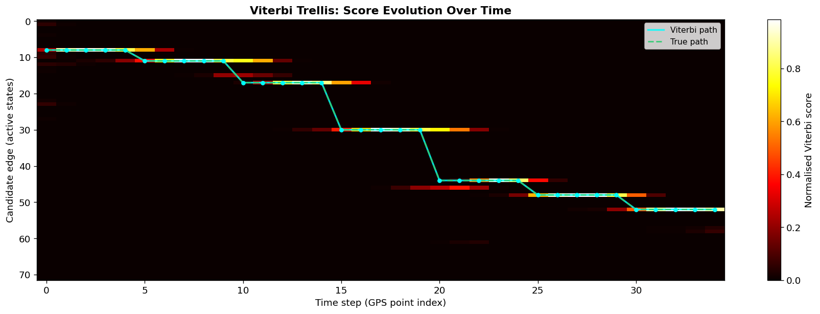
The key property of Viterbi is that this backward path is globally optimal, no other edge sequence has a higher joint probability under the HMM. This is different from greedy matching, which finds a local optimum at each step.

Step-by-Step Implementation

Step 1: Build the Road Graph

Load the road network and explode each edge into segments. Working at the segment level rather than the edge level gives precise snapping locations within long edges.

import osmnx as ox
import numpy as np
from scipy.sparse import csr_matrix

# Load road network for an area
G = ox.graph_from_place("Tel Aviv, Israel", network_type="drive")
nodes, edges = ox.graph_to_gdfs(G)

# Explode each edge into 2-point segments
segments = []
for (u, v, k), row in edges.iterrows():
    coords = list(row.geometry.coords)
    for i in range(len(coords) - 1):
        segments.append({
            "edge_id": (u, v, k),
            "start": coords[i],
            "end": coords[i+1],
            "bearing": compute_bearing(coords[i], coords[i+1])
        })

Step 2: Build a Spatial Index

Use a KD-tree or R-tree over segment midpoints for fast nearest-neighbor lookup.

from scipy.spatial import cKDTree

midpoints = np.array([(s["start"][0] + s["end"][0]) / 2,
                       (s["start"][1] + s["end"][1]) / 2]
                      for s in segments])
spatial_index = cKDTree(midpoints)

Step 3: Compute Emission Probabilities

For each GPS point, query the spatial index, then compute per-segment emission probabilities.

def emission_probabilities(gps_point, max_distance=350, k=400):
    dists, idxs = spatial_index.query(
        [gps_point.lon, gps_point.lat], k=k, distance_upper_bound=max_distance
    )
    valid = dists < max_distance
    dists, idxs = dists[valid], idxs[valid]

    segment_bearings = np.array([segments[i]["bearing"] for i in idxs])
    angle_diff = np.radians(np.abs(segment_bearings - gps_point.heading))
    heading_penalty = 1.0 - np.cos(angle_diff)

    probs = np.exp(-0.3875 * dists - 8.0 * heading_penalty)

    # Keep only the best segment per edge
    edge_ids = [segments[i]["edge_id"] for i in idxs]
    return best_per_edge(edge_ids, probs)

Step 4: Build the Transition Matrix

Precompute a sparse transition matrix over all edges in the graph.

rows, cols, data = [], [], []
avg_gps_interval_m = 15.0  # expected distance between GPS samples in meters

for edge_idx, (u, v, k) in enumerate(all_edges):
    edge_length = edges.loc[(u, v, k), "length"]
    move_prob = min(avg_gps_interval_m / edge_length, 0.5)

    # Self-loop
    rows.append(edge_idx); cols.append(edge_idx)
    data.append(1.0 - move_prob)

    # Neighbors
    neighbors = get_neighbors(G, v, edge_bearings[edge_idx])
    angles = np.array([a for _, a in neighbors])
    weights = np.exp(-3.0 * np.abs(angles))
    probs = (move_prob * weights) / weights.sum()

    for (nbr_idx, _), p in zip(neighbors, probs):
        rows.append(edge_idx); cols.append(nbr_idx)
        data.append(p)

transition = csr_matrix((data, (rows, cols)), shape=(N, N))

Step 5: Run the Viterbi Forward Pass

def viterbi(gps_trace):
    # Initialize with first point
    first_emissions = emission_probabilities(gps_trace[0])
    scores = dict(first_emissions)          # edge_idx -> probability
    back_ptrs = [{} for _ in gps_trace]    # back_ptrs[t][edge] = predecessor edge

    for t, gps_point in enumerate(gps_trace[1:], 1):
        next_scores = {}
        emissions = emission_probabilities(gps_point)

        for prev_idx, prev_score in scores.items():
            row = transition.getrow(prev_idx)
            for nbr_idx, trans_prob in zip(row.indices, row.data):
                candidate = prev_score * trans_prob
                if nbr_idx not in next_scores or candidate > next_scores[nbr_idx][0]:
                    next_scores[nbr_idx] = (candidate, prev_idx)

        scores = {}
        for edge_idx, (score, pred) in next_scores.items():
            if edge_idx in emissions:
                scores[edge_idx] = score * emissions[edge_idx]
                back_ptrs[t][edge_idx] = pred

        # Normalize to prevent underflow
        if scores:
            max_score = max(scores.values())
            scores = {k: v / max_score for k, v in scores.items()}

    return scores, back_ptrs

Step 6: Backtrack the Optimal Path

def backtrack(scores, back_ptrs):
    # Start from the best final state
    best_final = max(scores, key=scores.get)
    path = [best_final]

    for t in range(len(back_ptrs) - 1, 0, -1):
        path.append(back_ptrs[t][path[-1]])

    return list(reversed(path))

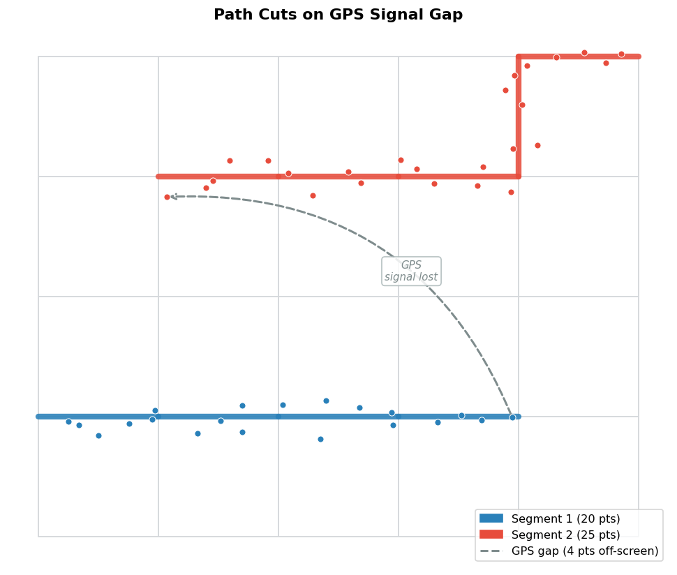
Handling GPS Gaps: Path Cuts

GPS traces in production are messy. Signals drop in tunnels, drivers pass through unmapped areas, and sometimes there are long gaps between observations. A continuous HMM would struggle: once the probability distribution becomes too diffuse, the backtracking produces unreliable results.

The solution is explicit path cutting. After each Viterbi step, check the total probability of the current state vector. If it falls below a threshold (e.g., exp(-50)), treat the current point as a new start: save the completed segment, then re-initialize the Viterbi state with only the current point’s emissions.

MIN_PROBABILITY = np.exp(-50)

total_score = sum(scores.values())
if total_score < MIN_PROBABILITY:
    completed_paths.append(backtrack(scores, back_ptrs[:t]))
    scores = emission_probabilities(gps_trace[t])
    back_ptrs = back_ptrs[t:]

This means the output can be a sequence of independent path segments rather than one continuous trace, which is often exactly what you want. A GPS gap produces a clean break in the matched route rather than a confused interpolation.

How It Compares to Greedy Matching

The Viterbi snapper solves a fundamentally harder problem than the greedy algorithms from the earlier series. Instead of matching individual points, it matches full sequences. The tradeoffs:

Accuracy: The biggest win is at the route level, not the point level. Point-level accuracy improvements are modest, the HMM doesn’t improve noisy GPS measurements. But the sequence of matched edges is far more coherent. Turns happen at the right places. The algorithm doesn’t jump between parallel roads. There are no isolated mismatches surrounded by correct ones.

Cost: Computing the transition matrix is a one-time cost proportional to graph size. The per-route Viterbi forward pass is sequential - each step depends on the previous one. The sparse representation keeps this tractable, but it’s harder to parallelize than greedy matching.

Global vs. local: The HMM uses global information. Every GPS point influences every other point’s matching through the back-pointer chain. A cluster of GPS points that clearly belongs to one edge provides evidence for the correct snapping of the ambiguous points nearby. Greedy algorithms can’t do this.

Summary

The Viterbi snapper replaces greedy, point-by-point map matching with a principled probabilistic framework. By modeling GPS observations as noisy emissions from hidden road states and computing optimal transitions across the road network topology, it finds the most likely edge sequence for the entire route in one pass.

The key ingredients:

• HMM: road edges as hidden states, GPS points as observations
• Emission probability: exponential decay in distance and heading misalignment
• Transition probability: graph connectivity + turn angle preference + stay/move balance
• Viterbi: dynamic programming forward pass + backtracking for global optimum
• Path cuts: graceful handling of GPS gaps and signal loss

Resources

References

[1] Newson, Paul, and John Krumm. “Hidden Markov map matching through noise and sparseness.” Proceedings of the 17th ACM SIGSPATIAL international conference on advances in geographic information systems. 2009.

[2] Viterbi, A. “Error bounds for convolutional codes and an asymptotically optimum decoding algorithm.” IEEE Transactions on Information Theory 13.2 (1967): 260-269.

[3] Rabiner, Lawrence R. “A tutorial on hidden Markov models and selected applications in speech recognition.” Proceedings of the IEEE 77.2 (1989): 257-286.