Map Matching Part 3 - Matching Algorithms
This series of articles will look into the subject of map matching, providing foundational knowledge. It examines the core concepts and inherent challenges within this domain, and details a comprehensive process for generating a synthetic dataset. The discussion then extends to exploring various map matching algorithms and a comparative evaluation of their performance, utilizing the dataset constructed.
Map Matching Algorithms
With our dataset generated, we can now implement and evaluate several map-matching algorithms to understand their respective strengths and weaknesses. We will explore four distinct approaches, starting from a simple baseline and progressively building in complexity:
- Baseline Matching
- Weighted Matching
- Topological Matching
- Hybrid Matching
This sequence was chosen because the algorithms are straightforward, grounded in solid theoretical principles, and build upon one another, creating a clear and logical progression. Importantly, these methods are known to produce strong results in practice [1].
Before diving into the solutions, let’s formally redefine the problem:
Annotations:
- X - longitude
- Y - latitude
- B - bearing
- H - heading
- A - accuracy
- E - edge in the graph
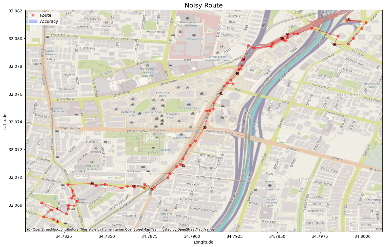
Given GPS samples that contains: Xnoisy, Ynoisy, Bnoisy, Hnoisy, Aaccuracy Our objective is to find the corrected coordinates: Xpred, Ypred, and the most likely road segment: Epred
The primary goals are: To assign the point to the correct road segment in the graph:
Epred = Eactual
To minimize the geometric distance between the predicted point and the true point:
Min(((Xpred - Xactual) ** 2 + (Ypred - Yactual) ** 2)** 0.5)
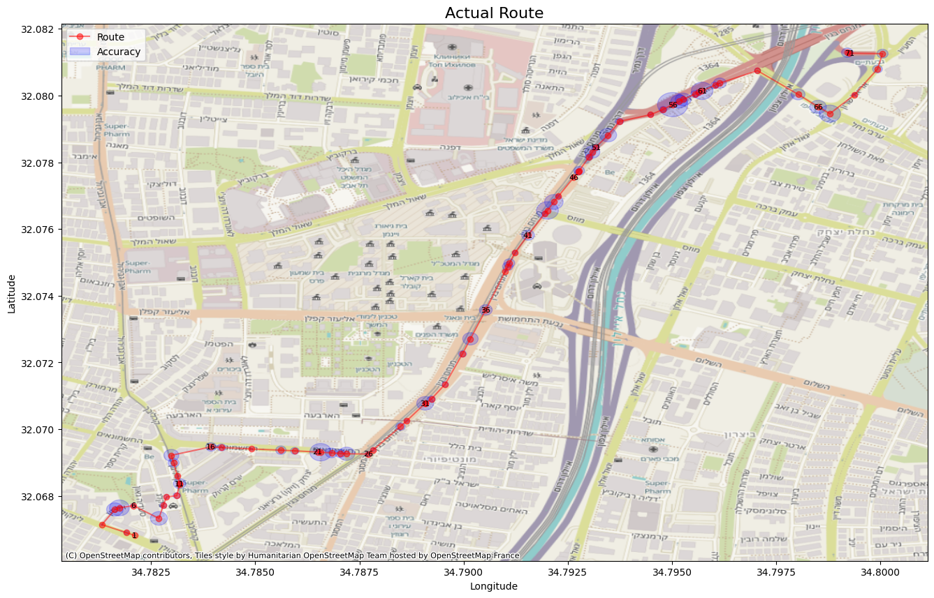
In simple terms, our mission is to accurately snap each noisy GPS point to the correct road on the map, ensuring the corrected location is as close as possible to the vehicle’s actual position. Easy peasy.
Evaluation
To evaluate our algorithms, we’ll use a multiple metrics approach that assesses performance at both the individual point level and the overall route level. Our three key metrics:
- Point-level Accuracy (Classification): This is the percentage of GPS samples correctly matched to their true edge. It tells us how often the algorithm gets the right answer.
- Point-level Error (Regression): This measures the average geometric distance (in meters) between the algorithm’s predicted point and the actual location. This quantifies how wrong the matches are.
- Route Similarity (Structural): Since a trajectory is a connected sequence, we also need a metric that evaluates the entire route’s structural integrity. Point-level metrics alone can be misleading; an algorithm might get 99% of points right but place one on a completely different highway.
For route-level evaluation, we’ll use a modified Levenshtein Distance [2]. This algorithm measures the difference between two sequences by counting the minimum number of single-edge “edits” (insertions, deletions, or substitutions) required to change one sequence into the other.
Before applying the metric, we perform a crucial preprocessing step: we compress both the actual and predicted routes by removing consecutive duplicates. For example, a route (1, 1, 1, 2, 2, 3) becomes (1, 2, 3). This is necessary because a vehicle generates multiple GPS samples while traversing a single long road segment.
Lets have a quick example, assuming the actual route is: 1, 1, 1, 2, 2, 2, 3, 2, 4. And our predicted route is: 1, 1, 2, 2, 1, 3, 3, 4. We’ll use our modification to exclude consecutive duplicates and turn it into: 1, 2, 3, 2, 4 and 1, 2, 1, 3, 4.
The first two edges (1 and 2) match perfectly. (0 edits) At the third position, the actual route has edge 3 while the predicted has 1. This requires one substitution. (1 edit) At the fourth position, the actual route has edge 2 while the predicted has 3. This requires a second substitution. (2 edits) The final edge (4) matches.
The total Levenshtein distance is 2. To make this value comparable across routes of different lengths, we normalize it into a score where 1 indicates a perfect match:
Lscore = 1 - (Ldistance / Max(Lenpredicted, Lenactual))
We evaluate every algorithm on 1000 routes from an augmented dataset we created in the previous article.
Base Class
To ensure a consistent structure, all algorithms are implemented on top of a single abstract base class called MatchingAlgorithm. This class manages two essential components: a graph attribute, holding the igraph.Graph road network we’ve discussed, and the index. The index is an STRtree provided by the shapely package, a data structure that enables highly efficient spatial queries on geometric objects, allowing us to quickly find nearby road segments for any given GPS point [3].
Each sample is matched using the following procedure:
- Extract the sample’s details: longitude, latitude, heading/bearing, and accuracy.
- Project the point from geographic coordinates to a local Cartesian system for accurate distance calculations.
- Identify a set of candidate road edges that are most likely to be the correct match.
- Score and select the single best candidate from this set based on specific criteria.
- Calculate the point’s perpendicular projection onto the selected edge geometry.
- Determine the final matched coordinates on that edge.
- Revert the final coordinates from the local system back to the original geographic system.
While most of these steps are shared, the “secret sauce” of each algorithm lies in Steps 3 and 4. The unique logic used to find, score, and rank candidate edges is what distinguishes the map matching algorithms in this article.
Baseline Algorithm
Every good analysis starts with a benchmark. A baseline algorithm serves as a fundamental point of comparison, allowing us to objectively measure the performance improvements offered by more sophisticated solutions. For our baseline, we’ll implement the most intuitive approach: a purely geometric match.
Translating this logic into our base implementation is just as simple: the get_candidates method is overridden to find and return only the single closest edge.
Since the list of candidates will always contain exactly one item, the find_best_match method simply selects it without needing any complex scoring logic.
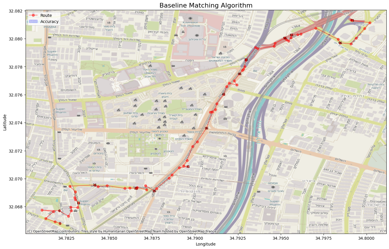
Accuracy: 0.47599 Distance: 16.01573 Lavenshtein: 0.50584
Weighted Matching
Moving beyond our simple baseline, the first real technique we’ll explore is Weighted Matching. The core idea is to create a more intelligent scoring system by combining multiple metrics. Instead of relying solely on distance, we’ll evaluate each candidate edge based on a weighted score that considers distance and bearing with the vehicle’s movement.
First, we select a pool of potential candidates using a dynamic search radius around the noisy GPS point. A robust method is to set this radius to three times the reported accuracy, as this covers over 99.7% of the probable locations for the vehicle (see previous map matching article for more information):
Dcandidates = Anoisy * 3
Next, each candidate in this pool is scored using a formula that combines two key factors: a Distance Score and a Bearing Score.
Ddiff = |(Y2 - Y1)Xnoisy - (X2 - X1)Ynoisy + X2Y1 - Y2X1| / ((Y2 - Y1) ** 2 + (X2 - X1) ** 2 ) ** 0.5
Bdiff = Min(|Bnoisy - Bedge|, 2pi - |Bnoisy - Bedge|)
Scorepred = 0.5 * (1 / Ddiff + 1) + 0.5 * ((cos(Bdiff) + 1) / 2)
Ddiff: This is the shortest perpendicular distance from the GPS point to the candidate edge (Yeah don’t worry about that, shapely has the implementation).
Bdiff: This measures the smallest angle between the vehicle’s bearing and the direction of the road segment, correctly handling the 360-degree wrap-around (e.g., the difference between 359° and 1° is 2°, not 358°).
These two components are then normalized and combined into a final score. For this implementation, we’ll assign them equal importance with a weight of 0.5 each.
The candidate with the highest Scorepred is selected as the best match.
One of the greatest strengths of this weighted system is its flexibility. You could easily incorporate another metric, like the difference between vehicle speed and the road’s speed limit, and adjust the weights to 0.33 for each. If you believe distance is more critical than bearing for your use case, you could change their respective weights to 0.7 and 0.3. This adaptability allows the algorithm to be fine-tuned for specific datasets and requirements.
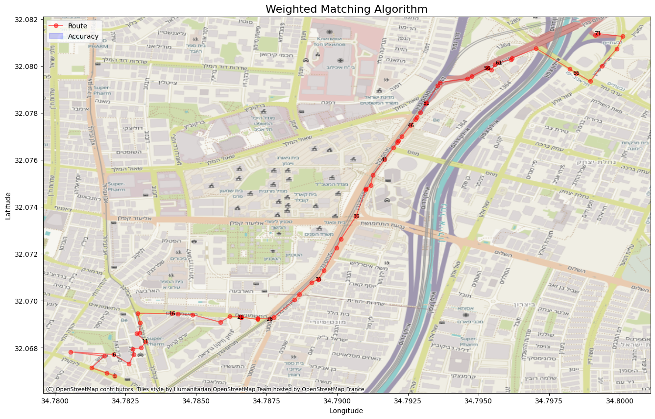
Accuracy: 0.658677 Distance: 13.40313 Lavenshtein: 0.68891
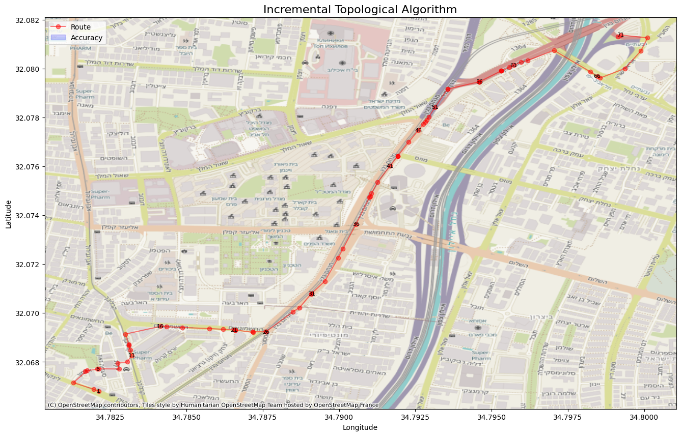
Topological Matching
Our Weighted Matching algorithm is a significant step up from the baseline, but it has a critical limitation: it treats every GPS point in isolation. Topological Matching remedies this by introducing the concept of memory. It leverages the fundamental structure of the road network to understand that a vehicle’s next position is highly dependent on its current one. Simply put, a car on edge A is far more likely to next be on an adjacent edge B than on a disconnected edge Z across town.
To implement it, we first maintain the state of each route by remembering the most recently matched road segment. For each new GPS point, we calculate the Weighted Score for all candidate edges as before, but then we add a topology_bias to reward candidates that are topologically sensible.
The rules for the bias are as follows:
- If a candidate edge is the same as the previous edge, it receives a high bias: + 0.2
- If a candidate edge is directly connected to the previous edge, it receives a medium bias: + 0.1
- If a candidate is disconnected from the previous edge, it receives no bias: + 0.0
The final score is then calculated as: Final Score = Weighted Score + topology_bias The candidate with the highest final score is chosen as the best match.
Accuracy: 0.57710 Distance: 14.35921 Lavenshtein: 0.71596
A Note on Design: Bias vs. Factor
I initially experimented with a multiplicative topology_factor instead of an additive bias (e.g., multiplying the score by 1.5, 1.2, or 1.0, respectively). However, I found this approach to be too aggressive. A multiplicative factor can disproportionately amplify already high scores, potentially locking the algorithm onto a nearby highway even if a topologically correct local road is a better fit. An additive bias provides a more gentle and stable “nudge” toward the correct path, leading to more robust results.
Results
| Algorithm Name | Accuracy | Distance | Lavenshtein |
|---|---|---|---|
| Baseline | 0.47599 | 16.01573 | 0.50584 |
| Weighted | 0.65867 | 13.40313 | 0.68891 |
| Topological | 0.57710 | 14.35921 | 0.71596 |
Summary
In this series, we embarked on a comprehensive journey to build an effective map-matching solution from the ground up. We moved from theory and synthetic data generation to implementing and evaluating a progression of algorithms. This process revealed a critical insight: the “best” approach is not one-size-fits-all. The optimal strategy depends on the context, particularly the quality of the GPS signal, and requires balancing the trade-offs between different evaluation metrics like point-level accuracy and overall route integrity.
While this series provides a thorough foundation, the world of location intelligence is vast. For instance, performance can be enhanced by incorporating additional sensor data, such as signals from nearby WiFi networks or readings from a phone’s accelerometer and magnetometer. You can also implement even more advanced techniques, such as Incremental Look-Ahead algorithms or Sliding-Window Hidden Markov Models (HMMs).
But for now, this article concludes the map matching series.
Appendix: Results Analysis & Bonus Algorithm
We can see that the collected results match our predictions regarding the success of each algorithm, with one key exception: the performance of the Weighted algorithm compared to the Topological algorithm in certain metrics. This outcome could be explained by several reasons: a bug in the implementation, a flaw in the algorithm’s logic, or some special cases where the topological approach fails.
Since I’m the writer of the article, so obviously there are no bugs in my code (although reality is often disappointing) and the theory that providing more structural information should lead to better results, we’re left to explore the specific cases where this algorithm might perform worse than the simpler Weighted algorithm.
Let’s re-think the implementation. There are two main differences between our “advanced” algorithms and the baseline: candidate selection and scoring. Candidate selection is based on distance, but it uses a dynamic parameter: the accuracy of each GPS sample to define the search radius. Scoring first adds the bearing and distance difference (used in both Weighted and Topological) and then, for the Topological algorithm, we add the topology_bias. We can work under the assumption that this bias, which rewards physically sensible paths, shouldn’t “hurt” our score.
Let’s take another look at the metrics, broken down by accuracy:
High Accuracy (3m - 15m error)
Weighted Matching: Distance: 7.68, Accuracy: 0.7295
Incremental Topological: Distance: 8.96, Accuracy: 0.6472
Medium Accuracy (15m - 30m error)
Weighted Matching: Distance: 21.05, Accuracy: 0.5291
Incremental Topological: Distance: 23.88, Accuracy: 0.4291
Low Accuracy (30m - 60m error)
Weighted Matching: Distance: 48.69, Accuracy: 0.3327
Incremental Topological: Distance: 40.07, Accuracy: 0.3430
Very Low Accuracy (60m - 90m error)
Weighted Matching: Distance: 85.87, Accuracy: 0.1969
Incremental Topological: Distance: 55.03, Accuracy: 0.2767
You’ll notice a clear trend: when accuracy is high, Weighted Matching outperforms the Topological algorithm. When accuracy is low, the reverse is true. Let’s try to explain this:
When accuracy is high → The candidate set is small, and the distance differences between them are minimal. This gives the bearing difference a higher impact. In this delicate balance, adding the topology_bias can be too influential, causing the algorithm to repeat the same edge when it should be making a turn.
When accuracy is low → The candidate set is large and scattered. The distance differences are significant. Here, the topology_bias is extremely useful, acting as a powerful filter to eliminate candidates that are not connected to our current route.
In other words, the topology_bias helps filter down a large, noisy set of candidates to only those that follow the route’s logic.
Therefore, I’ve implemented one more algorithm: HybridMatching. This approach simply selects which matching logic to use based on the provided accuracy for each sample.
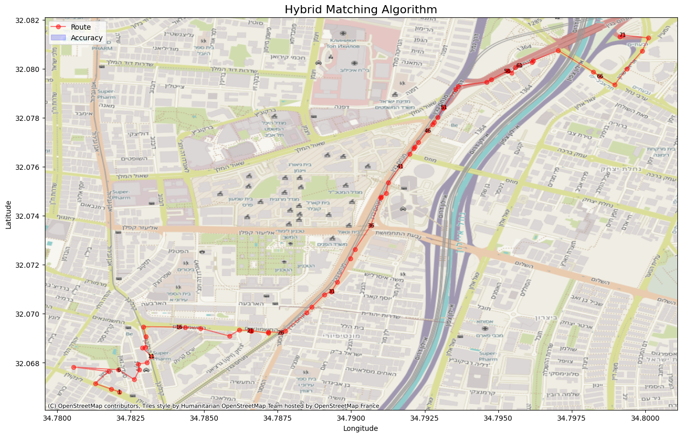
Accuracy: 0.65990 Distance: 12.75588 Lavenshtein: 0.69737
We can see that the point-level accuracy and distance error outperform all other algorithms. Interestingly, the Levenshtein score dropped slightly. This is because we deliberately allowed non-topological logic back into our algorithm for high-accuracy points, trading a small amount of perfect route structure for better point-by-point precision.
Resources
Code
https://github.com/ornachmias/map_matching
References
[1] Quddus, Mohammed A., Washington Y. Ochieng, and Robert B. Noland. “Current map-matching algorithms for transport applications: State-of-the art and future research directions.” Transportation research part c: Emerging technologies 15.5 (2007): 312-328
[2] https://en.wikipedia.org/wiki/Levenshtein_distance
[3] Leutenegger, Scott T., Mario A. Lopez, and Jeffrey Edgington. “STR: A simple and efficient algorithm for R-tree packing.” Proceedings 13th international conference on data engineering. IEEE, 1997.