Improving Navigation Performance Using a Hierarchical Graph
Introduction
If you’ve ever faced the challenge of writing your own navigation system, you’ve likely considered one of two solutions: either using an open-source system such as OSRM or Valhalla, or using OSM data to generate a graph and applying graph theory algorithms for navigation. While I’m a major advocate of open-source solutions, they sometimes have significant limitations (e.g., they cannot dynamically change edge weights, which set the actual time passing through a specific road, and instead rely instead on predefined weights based on time windows). In most cases, you can overlook those limitations or make some small changes to the code base, but if those are non-negotiable, or if you just feel like writing your own thing, the main issue you’re going to face when writing production-level service is the performance.
In this post I’ll show you how we can improve the performance of the navigation on graph using simple algorithms provided by both osmnx and igraph packages to modify our original graph, and then build a new graph made from multiple modified graphs to gain the performance boost needed for a production-grade service, with minimal data loss.
(A quick note about the plots in this post - I’m only going to show a very small part of the graphs each time to make the visualizations as clear as possible, later on when testing performance I’ll increase the size of the graph.)
OSM Graph Structure
Before diving into the question of how to improve performance, let’s take a look at the graph provided by OSM. Basically, assuming you’re looking at the driving graph, every driving available road will be an edge, those edges are always straight lines. By that, we can understand that every intersection or curve of the road is a vertex. The OSM data file israel-and-palestine-latest.osm.pbf is a graph with 2314075 vertices and 4069559 edges.
osm = OSM(map_path)
nodes, edges = osm.get_network(nodes=True, network_type='driving')
nx_graph = osm.to_graph(nodes, edges, graph_type='networkx')
raw_graph = ig.Graph.from_networkx(nx_graph)
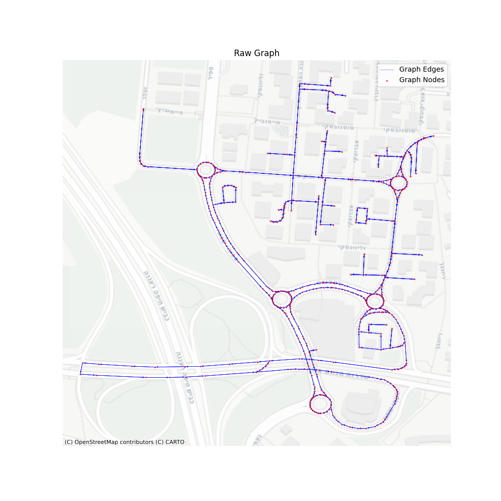
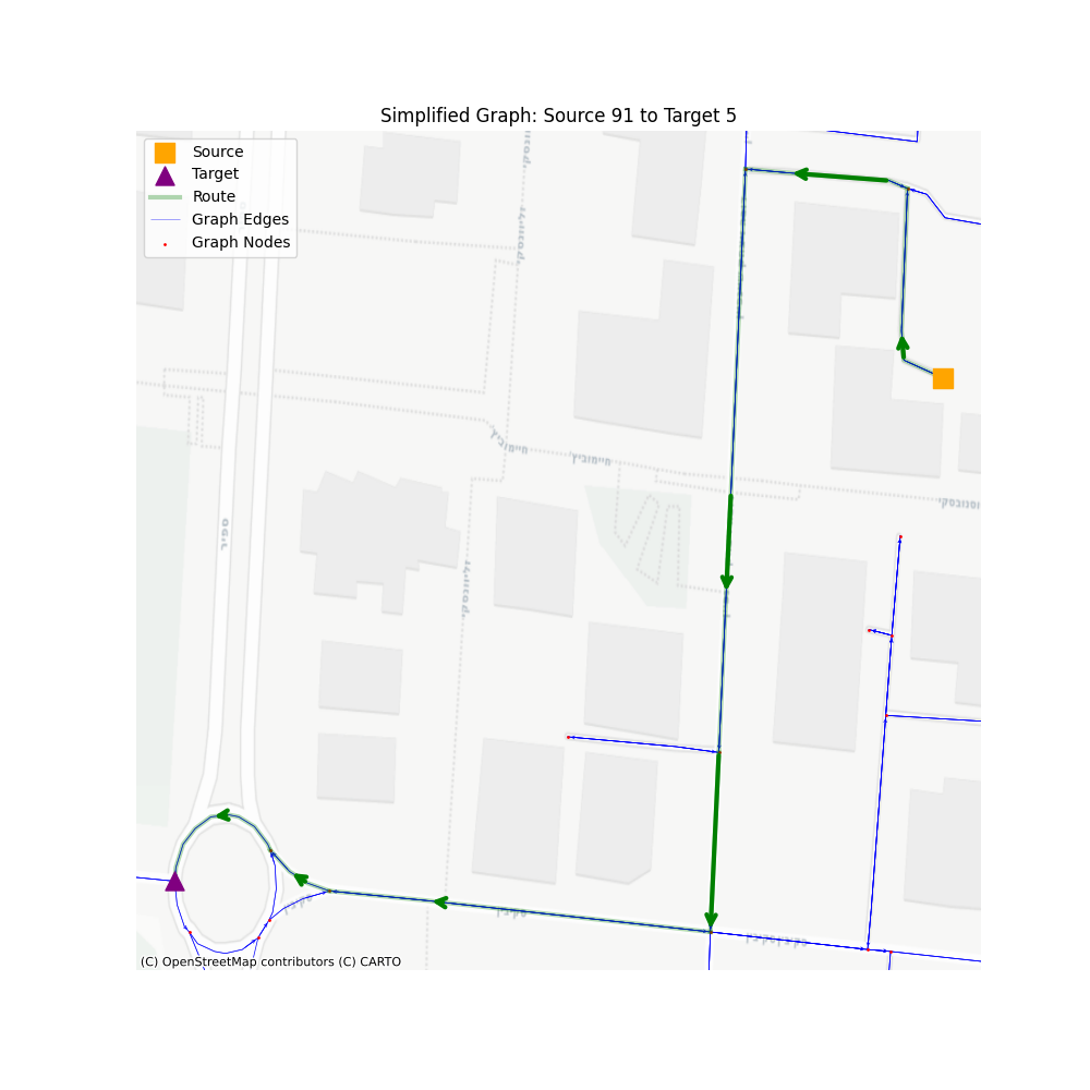
Now, at this point, finding the shortest path between two points is very easy, and will provide us with an extremely detailed route. We’ll simply use the “igraph” “get_shortest_path” method between our desired vertices, and a route will be available based on the vertices or edges in the path.
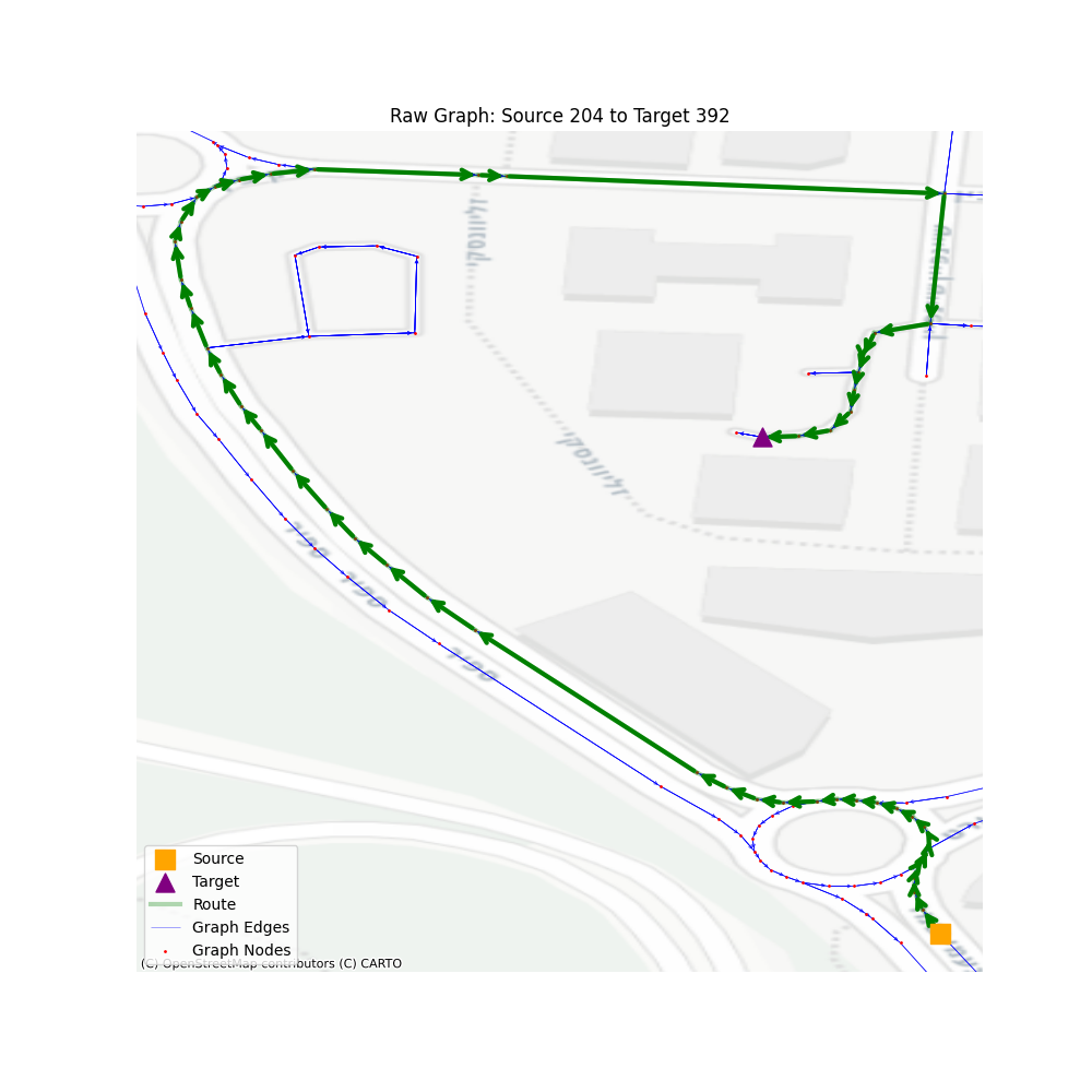
So, let’s take a look at the performance of such navigation when looking at a larger territory. I randomized 1000 sources and destinations, with some limitation on the number of steps in the path so we won’t accidentally use vertices that are on the same road, making the path finding trivial.
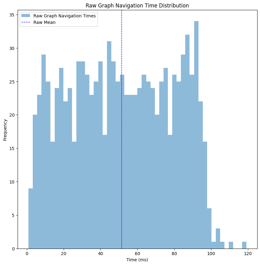
Looking at the performance histogram, things are looking pretty good - we got ourselves a mean time of ~50 milliseconds, and the max time is ~120 milliseconds, which is not bad for a production service. But let’s think about that for a second - I made the performance test on my laptop, making sure I’m running almost nothing except for that performance test. The requests were made sequentially, so the CPU was fully available for each request. When deploying such a thing to production, unless you have unlimited resources, such a thing won’t be possible. As an example, when trying to deploy this naive architecture into a service, we reached multiple seconds for each request. So from now on, we’ll continue the post assuming we care more about relative performance (comparing improvement between steps) instead of absolute values (evaluating success based on the milliseconds values).
Graph Simplification
The first observation you’ve probably noticed is that the graph is highly inefficient - every road is separated into multiple edges, thus containing so much more data than needed. The bigger the graph, the more time it takes to find the optimal shortest path. While the raw graph has its advantages (e.g. map matching is so much easier), in navigation this level of detail is redundant - the drivers won’t mind about every slight curve of the road, or if the sub-tag of the road changed. For data scientists, handling such a detailed graph is more difficult: when calculating durations from GPS data, there is much more room for errors when the roads are short, and we could also accidentally match points incorrectly to road segments.
So the first step in our hierarchical graph is to simplify the graph topology, without changing any of the geometries. That can be easily done using the package osmnx, specifically the method simplify_graph, which is based on “Topological Graph Simplification Solutions to the Street Intersection Miscount Problem.” publication by Boeing, G. This algorithm removes all nodes that are not intersections or dead-ends, and replaces them with an edge connected directly, while keeping the road shape using the geometry property.
nx_graph_simplified = ox.simplify_graph(nx_graph, track_merged=True)

Our graph now has 427001 vertices and 916380 edges, which reduced its size by about 80%. Let’s take a look at the performance of the get_shortest_path for this simplified graph.
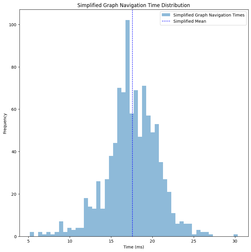
Just like that, we improved the time to ~18 milliseconds, a 60% improvement compared to the raw graph without any loss of necessary data.
From this point forward, this layer will be our baseline. We’ll create additional layers, where each layer will lose some of the information, but will gain us a performance boost.
Consolidate Intersections
Did you notice in the previous visualizations how roundabouts and intersections are represented using multiple nodes and edges? It makes sense, since we have a specific set of roads that intersect in a slightly different way in each case, based on the directions of the road and the type of intersection.
But when we want to navigate through a road network to calculate distance and ETA, we usually don’t care about such stuff, since as far as we are concerned - it’s just an intersection. When calculating ETA, I don’t really care how the driver crossed the intersection, only that he did.
This is where the consolidate_intersections in osmnx package come into play - it merges those intersections into a single node (based on provided tolerance value), and re-create the graph accordingly. The algorithm itself is also part of the G. Boeing (2025) paper we mentioned earlier, and it works by identifying and merging clusters of nearby nodes, often created by divided roads or traffic circles, which represent a single intersection in the real world. This consolidation algorithm will reduce our graph to 321243 vertices and 748246 edges, which is 24% smaller compared to the simplified graph.
Since we’re handling distance measurements, the graph should be projected before consolidated (you can read about it here), which is also a mandatory requirement by the package implementation of the algorithm.
nx_graph_consolidated = ox.project_graph(nx_graph_simplified, to_crs='EPSG:2039')
nx_graph_consolidated = ox.consolidate_intersections(nx_graph_consolidated, rebuild_graph=True, reconnect_edges=True)
nx_graph_consolidated = ox.project_graph(nx_graph_consolidated, to_crs='EPSG:4326')
While the route ETA and distance can be safely calculated using this graph, the main issue with this data simplification is that we do lose information here - the actual physical route. Meaning, if you wanted to create a nice UI to show the user how exactly he can navigate to the target - the nodes and edges won’t correlate with the underlying map. Let’s set aside this problem for now, and we’ll discuss it further on when we’ll build the full solution.
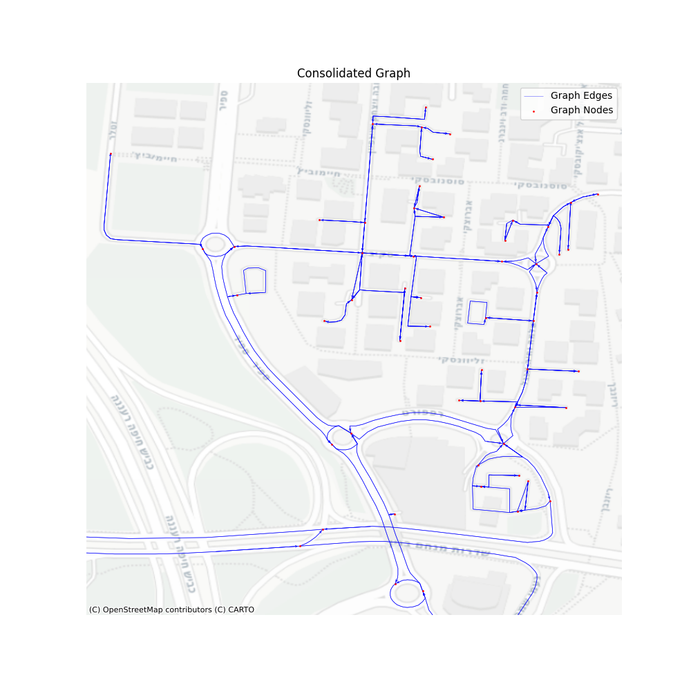
Let’s take a look at the performance of such a graph. Same territory, same map, only simplified and then consolidated.
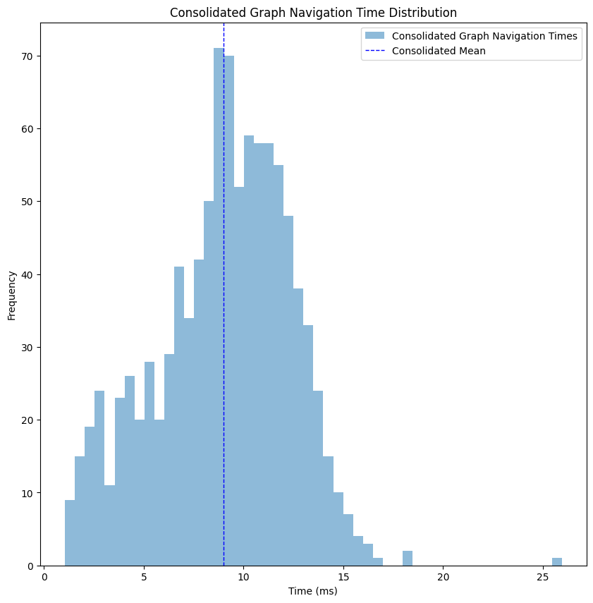
We improved from a mean of ~18 milliseconds to ~8 milliseconds, more than 50%, but with the loss of the actual geospatial route between the points.
Communities Graph
Having the consolidated graph on our hand, which supplies us the performance we needed, you might think that we should stop and deploy. But as I’ve mentioned before, this performance isn’t exactly what you’re going to see when handling a high volume of requests, so we need to somehow add some levels that will filter out unnecessary parts of the graphs.
Let’s look at a real example of a navigation request - a driver wants to get from one point in Tel-Aviv, Israel to another. Do we care about edges in other cities? Other countries? Even most of the edges in the same city are usually irrelevant to the route we’re looking for. Removing those parts of the graph will increase the performance of our overall algorithm, with minimal impact.
There are many methods to perform this kind of level - you can do it based on cities boundaries [1], or based on previous data you have [2], or even join multiple layers into several filtering levels. While you can do many combinations of filtering at this point - you have to be careful - too much filtering and you’ll lose data necessary to find the optimal path, too few and the overhead of the mapping will overcome the performance benefit.
As the title suggests, for this post I’ve chosen to generate communities using the Leiden algorithm. The Leiden algorithm discovers communities that have full connectivity within the community. While traditional methods sometimes made the mistake of loosely lumping items together just to form a group, Leiden introduces a refinement phase that ensures every discovered cluster is genuinely and densely connected. For our purposes, it’ll make sure that every point in the community has access to other locations in the same community, making sure that we don’t accidentally create islands of inaccessible vertices.
Even within the community discovery algorithms there are many options to choose from, but I’ve decided to choose Leiden due to its “safe” community generation. The major disadvantage is that the path might not be optimal. Some algorithms, such as infomap might find a more optimal community separation, but that requires an implementation of fallback in case of failure to filter things correctly, which I wish to keep out of scope for now.
partition = la.find_partition(consolidated_graph, la.CPMVertexPartition, resolution_parameter=0.05)
membership = partition.membership
communities_graph = consolidated_graph.copy()
communities_graph.contract_vertices(membership, combine_attrs=vertex_combiners)
communities_graph.simplify(combine_edges=edge_combiners, loops=True)
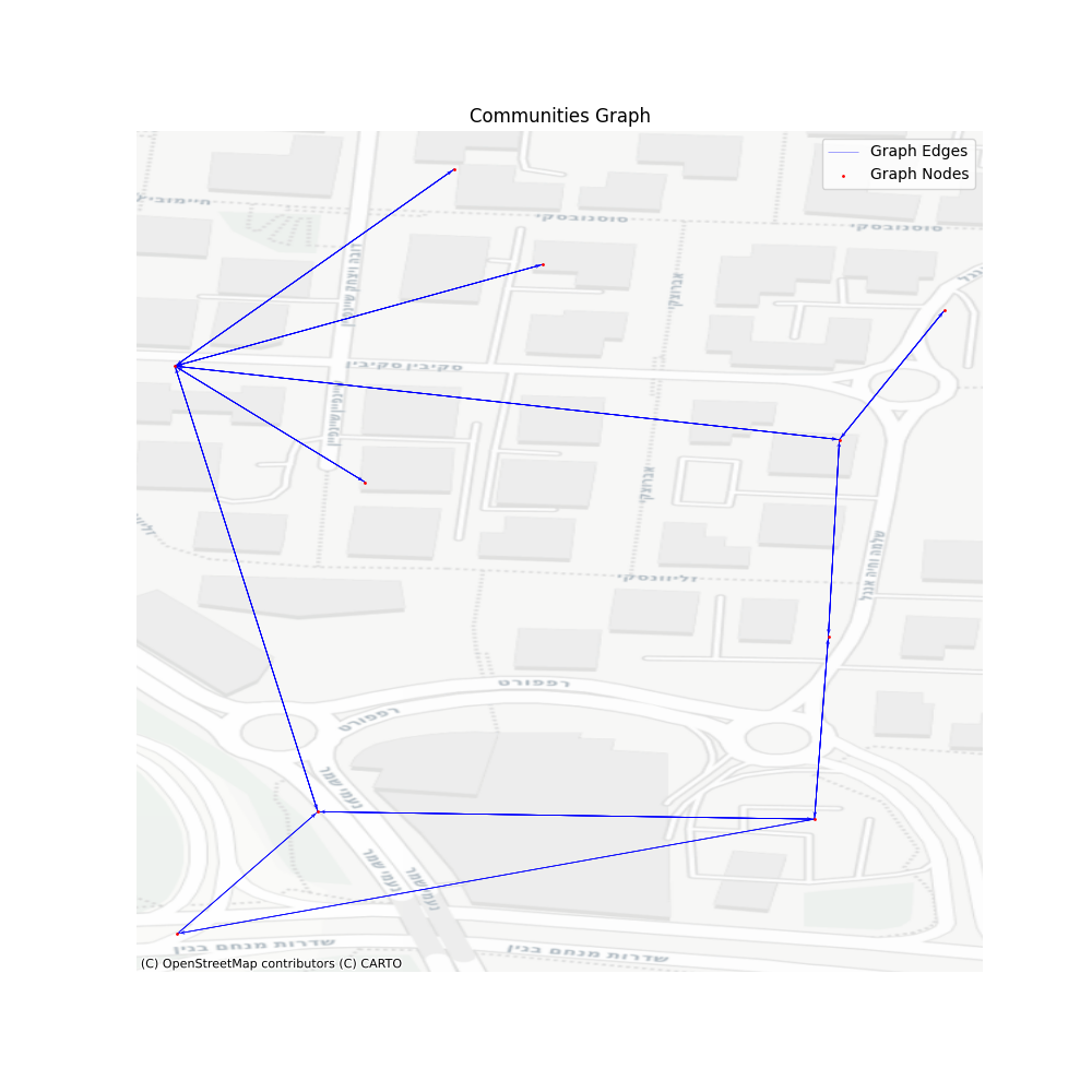
Looking at the graph we created we can see that it has almost nothing to do with the consolidated graph, but each vertex here represents an entire set of vertices. I’ve chosen a resolution of 0.05, which seems to satisfy the performance gain I wished to achieve. The output graph has 50597 vertices and 142989 edges, which is only 15% in size from our consolidated graph.
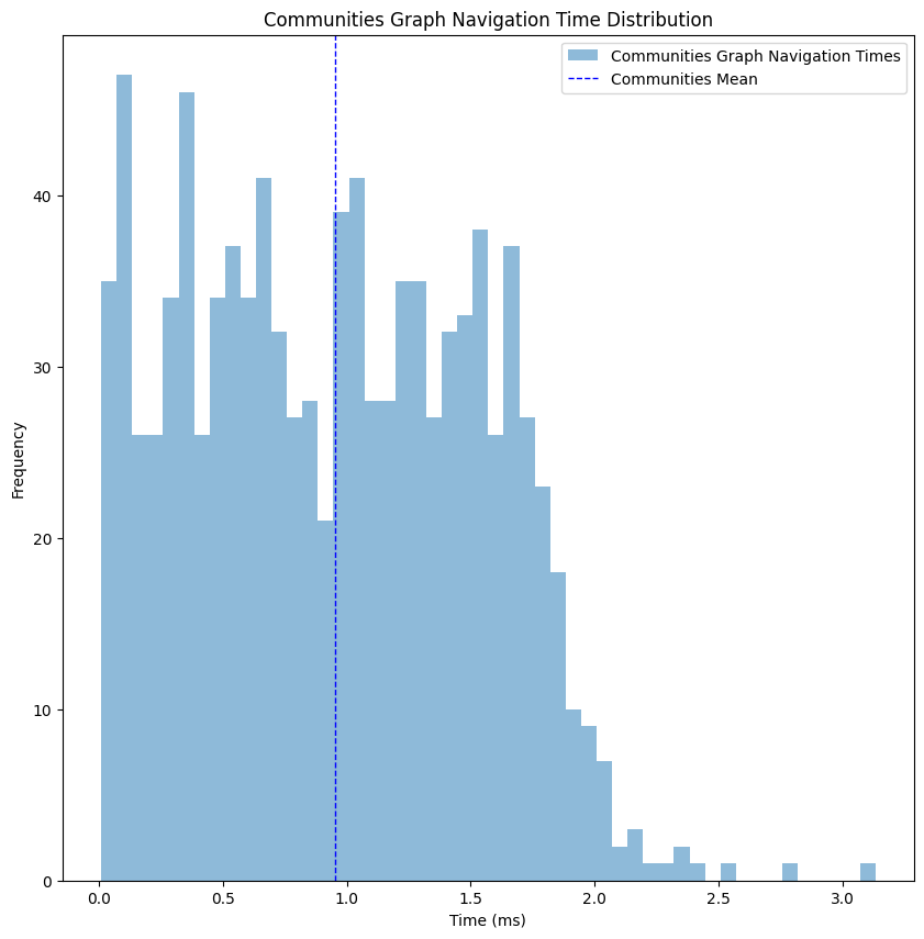
At this point the performance gain starts to get a bit obvious, but I wanted to have a full image of the steps taken. As you can see, we’ve dropped to an average performance of 1 millisecond, x8 improvement compared to the consolidated graph, meaning this kind of filtering will do the trick for now.
Building the Hierarchy
Up until now we’ve generated multiple graphs using different details resolution, where in one direction we improved the performance of navigating through it, while in the other we increased the number of details available though the found route. Our next step is to bind all of them together, so we could project one layer into the other, hence allowing us to move between them based on the level of detail we need at the moment.
The igraph package identifies edges and vertices using an index, but unfortunately this index cannot be consistent once we add or remove parts of the graph, so we need to overcome this challenge by creating our own mapping between those layers. The only limitations we’re facing are: 1. Achieving the mapping in O(1) performance, otherwise the overhead of moving between the graphs will cost us time instead of saving it. 2. Ensuring it supports vectorized operations, which, while not critical per se, will be vital for performance when deploying the service to handle multiple simultaneous navigation requests. Those two limitations are great, since the old scriptures mandate all data scientists to use only one data structure their entire career - pandas.DataFrame, which answers both of those requirements.
We’ll create multiple DataFrames, two for each movement we need (one way and the other): community to consolidated and consolidated to simplified, where the index will be our current vertex indices, and the value is the next vertex indices.
To get the transformation of the indices we’ll save on top of the graph in each step a “stable_index”, and when the graph will be transformed we’ll aggregate those properties together, and finally index them into a DataFrame. Let’s look at an example:
# Assuming we’ve just generated the community_graph
# and the consolidated graph had the same call to `set_stable_indices`
def set_stable_indices(graph, prefix):
   for v in graph.vs:
       v[f'{prefix}_stable_index'] = v.index

   for e in graph.es:
       e[f'{prefix}_stable_index'] = e.index


def flatten_if_needed(value):
   if isinstance(value, list) and len(value) > 0 and isinstance(value[0], list):
       return [item for sublist in value for item in sublist]
   return value

set_stable_indices(communities_graph, 'community')

# Unpack merged list of lists in indices and edges
stable_id_props = ['simplified_stable_index', 'consolidated_stable_index']
for v in communities_graph.vs:
   for prop in stable_id_props:
       if prop in v.attributes():
           v[prop] = flatten_if_needed(v[prop])

for e in communities_graph.es:
   for prop in stable_id_props:
       if prop in e.attributes():
           e[prop] = flatten_if_needed(e[prop])

def create_mapping(graph, current_stable_name, next_stable_name):
   current_vertices = graph.vs[current_stable_name]
   next_vertices = graph.vs[next_stable_name]


   current_to_next_vertices = pd.DataFrame(data={current_stable_name: current_vertices, next_stable_name: next_vertices}).set_index(current_stable_name)
   next_to_current_vertices = current_to_next_vertices.explode(next_stable_name)
   next_to_current_vertices = next_to_current_vertices.reset_index()
   next_to_current_vertices = next_to_current_vertices.groupby(next_stable_name)[current_stable_name].agg(list)

   return {'vertices': {'to_children': next_to_current_vertices, 'from_children': current_to_next_vertices}}

community_consolidated_mapping = create_mapping(communities_graph, 'community_stable_index', 'consolidated_stable_index')
This heavy (and slightly deformed) preprocessing is only done when we create the graph, then we can just save it aside and load it into the service. Notice that I kept the stable ids for both simplified and consolidated, so technically I can jump over layers in the architecture - from communities to simplified.
Navigating in Hierarchy
We created multiple graphs on top of each other, and we mapped the indices between those graphs. All that is left is to actually navigate through this entire pyramid of graphs. To do so, let’s assume we got as input the source and target from the simplified graph, and then we’ll perform the following:
- Map the simplified source/target to consolidated source/target
- Map the consolidated source/target to community source/target
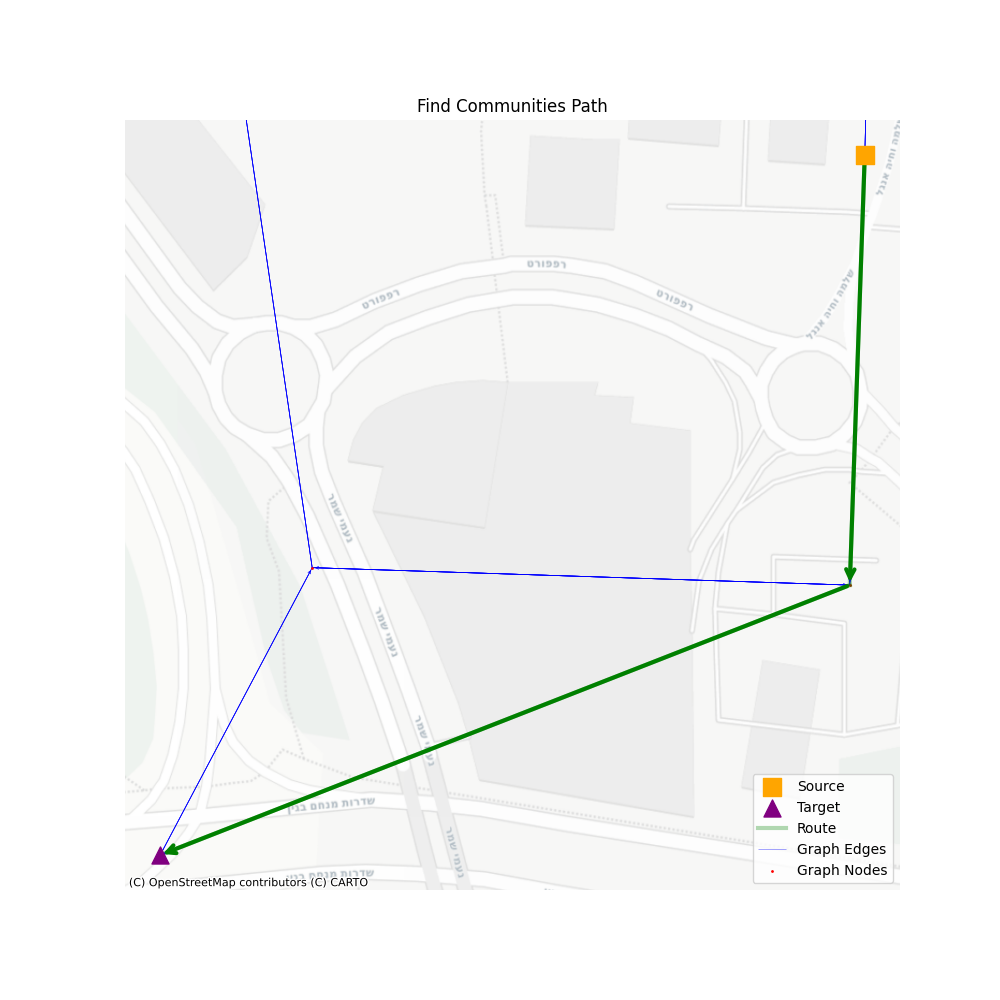
- Navigate in the communities graph and get communities path
- Map communities path into consolidated vertices
- Create a consolidated subgraph based on those vertices
- Find the consolidated subgraph source/target
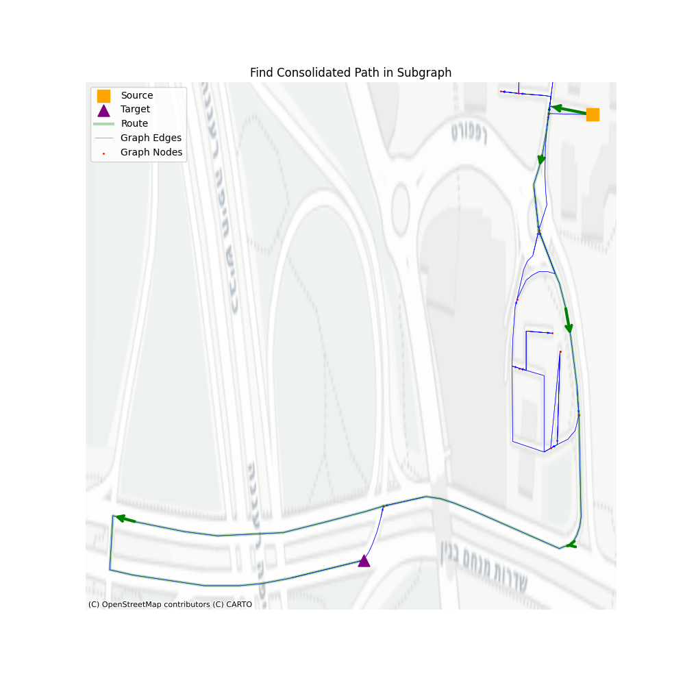
- Navigate through the consolidated subgraph and get consolidated subgraph path
- Map the consolidated subgraph path into consolidated graph vertices
- Map the consolidated graph vertices to simplified graph vertices
- Create a simplified subgraph from vertices
- Find the simplified source/target in the subgraph
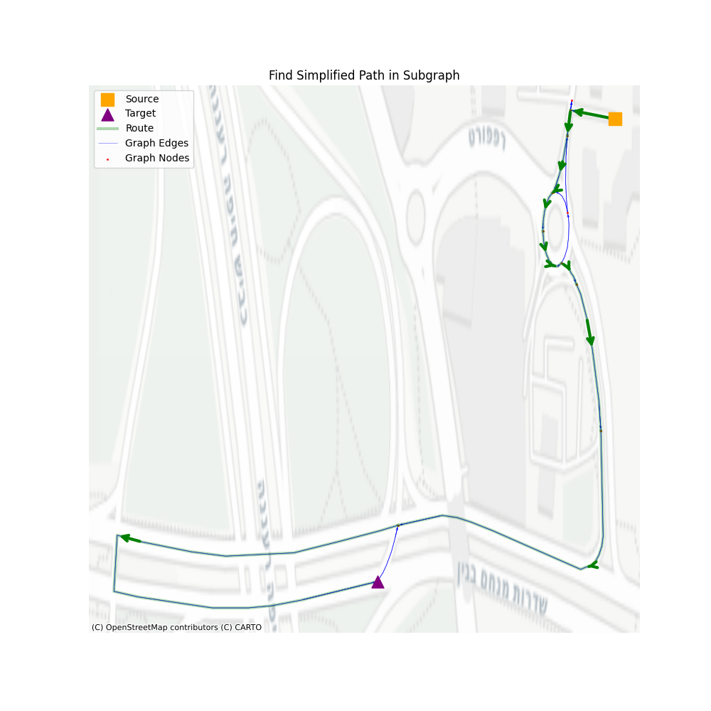
- Find a path in the simplified subgraph
Pretty long, right? Intuitively it seems so much more than simply navigating through the simplified graph and hoping for the best, but let’s take a look.
There are three main steps: 1. Navigate through communities, 2. Navigate through consolidated vertices, 3. Navigate through simplified graph vertices. All the rest are steps that help us remove unused vertices in the next level.
In terms of performance, let’s see how well we perform using a set of 1000 routes, with a minimum of 200 vertices in the simplified path.
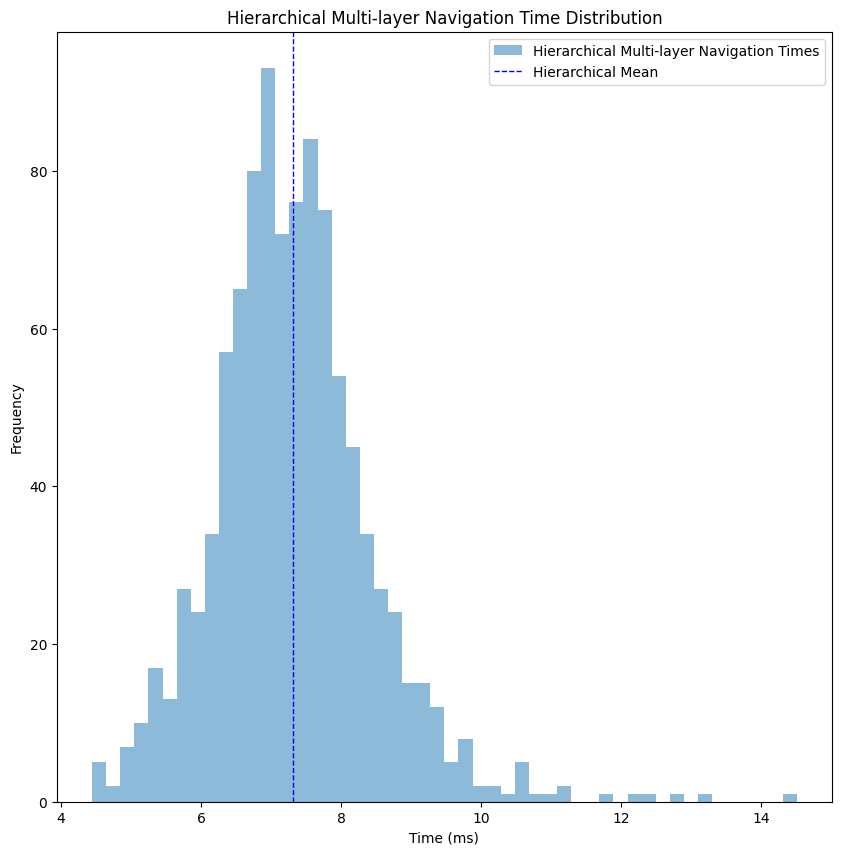
I’ve cleaned the two outliers to get a better look at the distribution, but even with them we average to ~11 milliseconds, which is almost 40% improvement from the simplified graph navigation, and almost the same as the consolidated graph navigation, but with all the additional geospatial details. In cases when we want to get only a consolidated path, for ETA and distance calculations, this average drops to ~7 milliseconds, an improvement of 12% compared to navigating through a consolidated graph alone.
Summary
Scaling a custom navigation engine requires more than just efficient algorithms, it requires efficient data structures. By transforming a raw OSM network into a hierarchical graph, we successfully balanced the need for geospatial data with the requirement for low-latency performance. Through the use of osmnx for simplification and consolidation and igraph for community detection, we reduced the search space by orders of magnitude. The final architecture resulted in a robust system capable of calculating detailed routes in low latency, proving that you don’t have to sacrifice detail for speed in production services.
Resources
Obligatory XKCD
References
[1] Jung, Sungwon, and Sakti Pramanik. “An efficient path computation model for hierarchically structured topographical road maps.”
[2] Yang, Xiaobo. “Directed-edge-based mining of regular routes for enhanced traffic pattern recognition from travel trajectories.”